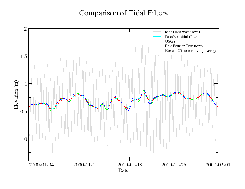
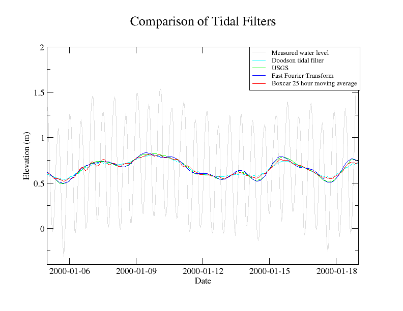
In general, the Fast Fourier Transform will create the best filtered data set.
You can ask for all of the filters to be output at once with the following command. Of course use your own data and definition file.
tappy.py analysis --outputts --filter usgs,transform,doodson,boxcar mayport_florida_8720220_data.txt mayport_florida_8720220_data_def.txt
Then look for the files outts_filtered_.dat where the is the name of the filter.
USGS
The USGS transform is a straight convolution. It is also known as PL33, since it has 33 values on either side of the the center value: 0.06215.
[-0.00027 -0.00114 -0.00211 -0.00317 -0.00427 -0.00537 -0.00641 -0.00735
 -0.00811 -0.00864 -0.00887 -0.00872 -0.00816 -0.00714 -0.0056  -0.00355
 -0.00097  0.00213  0.00574  0.0098   0.01425  0.01902  0.024    0.02911
  0.03423  0.03923  0.04399  0.04842  0.05237  0.05576  0.0585   0.06051
  0.06174  0.06215  0.06174  0.06051  0.0585   0.05576  0.05237  0.04842
  0.04399  0.03923  0.03423  0.02911  0.024    0.01902  0.01425  0.0098
  0.00574  0.00213 -0.00097 -0.00355 -0.0056  -0.00714 -0.00816 -0.00872
 -0.00887 -0.00864 -0.00811 -0.00735 -0.00641 -0.00537 -0.00427 -0.00317
 -0.00211 -0.00114 -0.00027]
Doodson
Doodson is also a convolution technique. The kernel is:
[1, 0, 1, 0, 0, 1, 0, 1, 1, 0, 2, 0, 1, 1, 0, 2, 1, 1, 2, 0, 2, 1, 1, 2, 0, 1, 1, 0, 2, 0, 1, 1, 0, 1, 0, 0, 1, 0, 1]
Boxcar
Boxcar is a strait moving average of 25 hours. This in effect makes it also a convolution technique with 25 values of 1/25.0.
Fast Fourier Transform
The FFT filtering process was described in ‘Removing Tidal-Period Variations from Time-Series Data Using Low Pass Filters’ by Roy Walters and Cythia Heston, 1981, in Physical Oceanography, Volume 12, pg 112. This article found that of the FFT transform, Godin, cosine-Lanczos squared filter, and cosine-Lanczos filter the FFT transform method performed the best.
After transform into the frequency domain zero out all frequencies lower than 30, leave untouched frequencies higher than 40 and linear ramp between 30 and 40. Transform the altered frequency domain series into the time-domain.
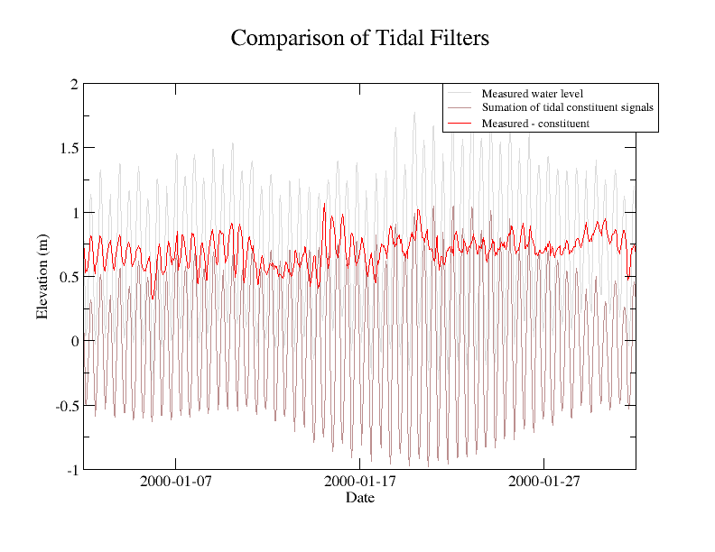
You might be tempted to simply subtract the sum of all the constituent signals from the original series. This doesn’t end up as nice as the tidal filters above.