tsgettoolbox and tstoolbox - Command Line Interface
‘tsgettoolbox nwis …’: Download data from the National Water Information System (NWIS)
This notebook is to illustrate the command line usage for ‘tsgettoolbox’ and ‘tstoolbox’ to download and work with data from the National Water Information System (NWIS). There is a different notebook to do the same thing from within a Python program called tsgettoolbox-nwis-api.
First off, always nice to remind myself about the options. Each sub-command has their own options kept consistent with the options available from the source service. The way that NWIS works is you have one major filter and one or more minor filters to define what sites you want.
[ ]:
tsgettoolbox nwis_dv --help
Let’s say that I want flow (parameterCd=00060) for site ‘02325000’. I first make sure that I am getting what I want by allowing the output to be printed to the screen. Note the pipe (’|’) that directs output to the ‘head’ command to display the top 10 lines of the time-series.
[14]:
tsgettoolbox nwis_dv --sites 02325000 --startDT '2000-01-01' --parameterCd 00060 | head
Datetime,USGS-02325000-00060
2000-01-01,82
2000-01-02,81
2000-01-03,80
2000-01-04,79
2000-01-05,75
2000-01-06,75
2000-01-07,74
2000-01-08,73
2000-01-09,75
Then I redirect to a file with “> filename.csv” so that I don’t have to wait for the USGS NWIS services for the remaining work or analysis.
[15]:
tsgettoolbox nwis_dv --sites 02325000 --startDT '2000-01-01' --parameterCd 00060 > 02325000_flow.csv
‘tstoolbox …’: Process data using ‘tstoolbox’
Now lets use “tstoolbox” to plot the time-series. Note the redirection again, this time for input as “< filename.csv”. Default plot filename is “plot.png”.
[16]:
tstoolbox plot < 02325000_flow.csv
‘tstoolbox plot’ has many options that can be used to modify the plot.
[17]:
tstoolbox plot --help
usage: tstoolbox plot [-h] [--ofilename <str>] [--type <str>] [--xtitle <str>]
  [--ytitle <str>] [--title <str>] [--figsize <str>] [--legend LEGEND]
  [--legend_names <str>] [--subplots] [--sharex] [--sharey] [--style <str>]
  [--logx] [--logy] [--xaxis <str>] [--yaxis <str>] [--xlim XLIM] [--ylim
  YLIM] [--secondary_y] [--mark_right] [--scatter_matrix_diagonal <str>]
  [--bootstrap_size BOOTSTRAP_SIZE] [--bootstrap_samples BOOTSTRAP_SAMPLES]
  [--norm_xaxis] [--norm_yaxis] [--lognorm_xaxis] [--lognorm_yaxis]
  [--xy_match_line <str>] [--grid GRID] [-i <str>] [-s <str>] [-e <str>]
  [--label_rotation <int>] [--label_skip <int>] [--force_freq FORCE_FREQ]
  [--drawstyle <str>] [--por] [--columns COLUMNS] [--invert_xaxis]
  [--invert_yaxis] [--plotting_position <str>]

Plot data.

optional arguments:
  -h | --help
      show this help message and exit
  --ofilename <str>
      Output filename for the plot. Extension defines the type, ('.png').
      Defaults to 'plot.png'.
  --type <str>
      The plot type. Defaults to 'time'.
      Can be one of the following:
      time
        standard time series plot

      xy
        (x,y) plot, also know as a scatter plot

      double_mass
        (x,y) plot of the cumulative sum of x and y

      boxplot
        box extends from lower to upper quartile, with line at the median.
        Depending on the statistics, the wiskers represent the range of
        the data or 1.5 times the inter-quartile range (Q3 - Q1)

      scatter_matrix
        plots all columns against each other

      lag_plot
        indicates structure in the data

      autocorrelation
        plot autocorrelation

      bootstrap
        visually asses aspects of a data set by plotting random selections of
        values

      probability_density
        sometime called kernel density estimation (KDE)

      bar
        sometimes called a column plot

      barh
        a horizontal bar plot

      bar_stacked
        sometimes called a stacked column

      barh_stacked
        a horizontal stacked bar plot

      histogram
        calculate and create a histogram plot

      norm_xaxis
        sort, calculate probabilities, and plot data against an x axis normal
        distribution

      norm_yaxis
        sort, calculate probabilities, and plot data against an y axis normal
        distribution

      lognorm_xaxis
        sort, calculate probabilities, and plot data against an x axis lognormal
        distribution

      lognorm_yaxis
        sort, calculate probabilities, and plot data against an y axis lognormal
        distribution

      weibull_xaxis
        sort, calculate and plot data against an x axis weibull distribution

      weibull_yaxis
        sort, calculate and plot data against an y axis weibull distribution

  --xtitle <str>
      Title of x-axis, default depend on type.
  --ytitle <str>
      Title of y-axis, default depend on type.
  --title <str>
      Title of chart, defaults to ''.
  --figsize <str>
      The 'width,height' of plot as inches. Defaults to '10,6.5'.
  --legend LEGEND
      Whether to display the legend. Defaults to True.
  --legend_names <str>
      Legend would normally use the time-series names associated with the input
      data. The 'legend_names' option allows you to override the names in
      the data set. You must supply a comma separated list of strings for
      each time-series in the data set. Defaults to None.
  --subplots
      boolean, default False. Make separate subplots for each time series
  --sharex
      boolean, default True In case subplots=True, share x axis
  --sharey
      boolean, default False In case subplots=True, share y axis
  --style <str>
      Comma separated matplotlib style strings matplotlib line style per
      time-series. Just combine codes in 'ColorLineMarker' order, for
      example r--* is a red dashed line with star marker.
      ┌──────┬─────────┐
      │ Code │ Color   │
      ├──────┼─────────┤
      │ b    │ blue    │
      ├──────┼─────────┤
      │ g    │ green   │
      ├──────┼─────────┤
      │ r    │ red     │
      ├──────┼─────────┤
      │ c    │ cyan    │
      ├──────┼─────────┤
      │ m    │ magenta │
      ├──────┼─────────┤
      │ y    │ yellow  │
      ├──────┼─────────┤
      │ k    │ black   │
      ├──────┼─────────┤
      │ w    │ white   │
      ╘══════╧═════════╛

      ┌─────────┬───────────┐
      │ Number  │ Color     │
      ├─────────┼───────────┤
      │ 0.75    │ 0.75 gray │
      ├─────────┼───────────┤
      │ ...etc. │           │
      ╘═════════╧═══════════╛

      ┌──────────────────┐
      │ HTML Color Names │
      ├──────────────────┤
      │ red              │
      ├──────────────────┤
      │ burlywood        │
      ├──────────────────┤
      │ chartreuse       │
      ├──────────────────┤
      │ ...etc.          │
      ╘══════════════════╛

      Color reference: <http://matplotlib.org/api/colors_api.html>
      ┌──────┬──────────────┐
      │ Code │ Lines        │
      ├──────┼──────────────┤
      │ •    │ solid        │
      ├──────┼──────────────┤
      │ --   │ dashed       │
      ├──────┼──────────────┤
      │ -.   │ dash_dot     │
      ├──────┼──────────────┤
      │ :    │ dotted       │
      ├──────┼──────────────┤
      │ None │ draw nothing │
      ├──────┼──────────────┤
      │ ' '  │ draw nothing │
      ├──────┼──────────────┤
      │ ''   │ draw nothing │
      ╘══════╧══════════════╛

      Line reference: <http://matplotlib.org/api/artist_api.html>
      ┌──────┬────────────────┐
      │ Code │ Markers        │
      ├──────┼────────────────┤
      │ .    │ point          │
      ├──────┼────────────────┤
      │ o    │ circle         │
      ├──────┼────────────────┤
      │ v    │ triangle down  │
      ├──────┼────────────────┤
      │ ^    │ triangle up    │
      ├──────┼────────────────┤
      │ <    │ triangle left  │
      ├──────┼────────────────┤
      │ >    │ triangle right │
      ├──────┼────────────────┤
      │ 1    │ tri_down       │
      ├──────┼────────────────┤
      │ 2    │ tri_up         │
      ├──────┼────────────────┤
      │ 3    │ tri_left       │
      ├──────┼────────────────┤
      │ 4    │ tri_right      │
      ├──────┼────────────────┤
      │ 8    │ octagon        │
      ├──────┼────────────────┤
      │ s    │ square         │
      ├──────┼────────────────┤
      │ p    │ pentagon       │
      ├──────┼────────────────┤
      │ •    │ star           │
      ├──────┼────────────────┤
      │ h    │ hexagon1       │
      ├──────┼────────────────┤
      │ H    │ hexagon2       │
      ├──────┼────────────────┤
      │ •    │ plus           │
      ├──────┼────────────────┤
      │ x    │ x              │
      ├──────┼────────────────┤
      │ D    │ diamond        │
      ├──────┼────────────────┤
      │ d    │ thin diamond   │
      ├──────┼────────────────┤
      │ _    │ hline          │
      ├──────┼────────────────┤
      │ None │ nothing        │
      ├──────┼────────────────┤
      │ ' '  │ nothing        │
      ├──────┼────────────────┤
      │ ''   │ nothing        │
      ╘══════╧════════════════╛

      Marker reference: <http://matplotlib.org/api/markers_api.html>
  --logx
      DEPRECATED: use '--xaxis="log"' instead.
  --logy
      DEPRECATED: use '--yaxis="log"' instead.
  --xaxis <str>
      Defines the type of the xaxis. One of 'arithmetic', 'log'. Default is
      'arithmetic'.
  --yaxis <str>
      Defines the type of the yaxis. One of 'arithmetic', 'log'. Default is
      'arithmetic'.
  --xlim XLIM
      Comma separated lower and upper limits (--xlim 1,1000) Limits for the
      x-axis. Default is based on range of x values.
  --ylim YLIM
      Comma separated lower and upper limits (--ylim 1,1000) Limits for the
      y-axis. Default is based on range of y values.
  --secondary_y
      Boolean or sequence, default False Whether to plot on the secondary y-axis
      If a list/tuple, which time-series to plot on secondary y-axis
  --mark_right
      Boolean, default True : When using a secondary_y axis, should the legend
      label the axis of the various time-series automatically
  --scatter_matrix_diagonal <str>
      If plot type is 'scatter_matrix', this specifies the plot along the
      diagonal. Defaults to 'probability_density'.
  --bootstrap_size BOOTSTRAP_SIZE
      The size of the random subset for 'bootstrap' plot. Defaults to 50.
  --bootstrap_samples BOOTSTRAP_SAMPLES
      The number of random subsets of 'bootstrap_size'. Defaults to 500.
  --norm_xaxis
      DEPRECATED: use '--type="norm_xaxis"' instead.
  --norm_yaxis
      DEPRECATED: use '--type="norm_yaxis"' instead.
  --lognorm_xaxis
      DEPRECATED: use '--type="lognorm_xaxis"' instead.
  --lognorm_yaxis
      DEPRECATED: use '--type="lognorm_yaxis"' instead.
  --xy_match_line <str>
      Will add a match line where x == y. Default is ''. Set to a line style
      code.
  --grid GRID
      Boolean, default True Whether to plot grid lines on the major ticks.
  -i <str> | --input_ts <str>
      Filename with data in 'ISOdate,value' format or '-' for stdin.
  -s <str> | --start_date <str>
      The start_date of the series in ISOdatetime format, or 'None' for
      beginning.
  -e <str> | --end_date <str>
      The end_date of the series in ISOdatetime format, or 'None' for end.
  --label_rotation <int>
      Rotation for major labels for bar plots.
  --label_skip <int>
      Skip for major labels for bar plots.
  --force_freq FORCE_FREQ
      Force this frequency for the plot. WARNING: you may lose data if not
      careful with this option. In general, letting the algorithm
      determine the frequency should always work, but this option will
      override. Use PANDAS offset codes,
  --drawstyle <str>
      'default' connects the points with lines. The steps variants produce
      step-plots. 'steps' is equivalent to 'steps-pre' and is maintained
      for backward-compatibility. ACCEPTS:
      ['default' | 'steps' | 'steps-pre' | 'steps-mid' | 'steps-post']

  --por
      Plot from first good value to last good value. Strip NANs from beginning
      and end.
  --columns COLUMNS
      Columns to pick out of input. Can use column names or column numbers. If
      using numbers, column number 1 is the first data column. To pick
      multiple columns; separate by commas with no spaces. As used in
      'pick' command.
  --invert_xaxis
      Invert the x-axis.
  --invert_yaxis
      Invert the y-axis.
  --plotting_position <str>
      'weibull', 'benard', 'tukey', 'gumbel', 'hazen', 'cunnane', or
      'california'. The default is 'weibull'.
      ┌────────────┬─────────────────┬───────────────────────┐
      │ weibull    │ i/(n+1)         │ mean of sampling      │
      │            │                 │ distribution          │
      ├────────────┼─────────────────┼───────────────────────┤
      │ benard     │ (i-0.3)/(n+0.4) │ approx. median of     │
      │            │                 │ sampling distribution │
      ├────────────┼─────────────────┼───────────────────────┤
      │ tukey      │ (i-1/3)/(n+1/3) │ approx. median of     │
      │            │                 │ sampling distribution │
      ├────────────┼─────────────────┼───────────────────────┤
      │ gumbel     │ (i-1)/(n-1)     │ mode of sampling      │
      │            │                 │ distribution          │
      ├────────────┼─────────────────┼───────────────────────┤
      │ hazen      │ (i-1/2)/n       │ midpoints of n equal  │
      │            │                 │ intervals             │
      ├────────────┼─────────────────┼───────────────────────┤
      │ cunnane    │ (i-2/5)/(n+1/5) │ subjective            │
      ├────────────┼─────────────────┼───────────────────────┤
      │ california │ i/n             │                       │
      ╘════════════╧═════════════════╧═══════════════════════╛

      Where 'i' is the sorted rank of the y value, and 'n' is the total number
      of values to be plotted.
      Only used for norm_xaxis, norm_yaxis, lognorm_xaxis, lognorm_yaxis,
      weibull_xaxis, and weibull_yaxis.
[18]:
tstoolbox plot --ofilename flow.png --ytitle 'Flow (cfs)' --title '02325000: FENHOLLOWAY RIVER NEAR PERRY, FLA' --legend False < 02325000_flow.csv
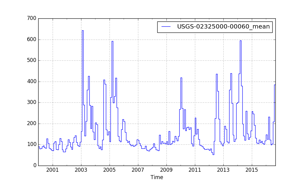
Monthly Average Flow
You can also use tstoolbox to make calculations on the time-series, for example to aggregate to monthly average flow:
[21]:
tstoolbox aggregate --groupby M --statistic mean < 02325000_flow.csv | head
Datetime,USGS-02325000-00060_mean
2000-01-31,80
2000-02-29,89.7931
2000-03-31,80.0323
2000-04-30,81.7667
2000-05-31,90.8387
2000-06-30,94.4
2000-07-31,85.9032
2000-08-31,83.0323
2000-09-30,128.067
[20]:
tstoolbox aggregate --groupby M --statistic mean < 02325000_flow.csv | tstoolbox plot --ofilename plot_monthly.png --drawstyle steps-pre