‘tstoolbox plot …’ using the command line interface

This notebook illustrates some of the plotting features of tstoolbox on the command line.

For detailed help type ‘tstoolbox plot –help’ at the command line prompt.

The available plot types are: time, xy, double_mass, boxplot, scatter_matrix, lag_plot, autocorrelation, bootstrap, histogram, kde, kde_time, bar, barh, bar_stacked, barh_stacked, heatmap, norm_xaxis, norm_yaxis, lognorm_xaxis, lognorm_yaxis, weibull_xaxis, weibull_yaxis

First, let’s get some data using tsgettoolbox

tsgettoolbox nwis_dv --sites 02233484 --startDT 2000-01-01 > 02233484.csv
tsgettoolbox nwis_dv --sites 02233500 --startDT 2000-01-01 > 02233500.csv

Let’s look at the top of the data files using the ‘head’ command.

head 02233484.csv 02233500.csv

==> 02233484.csv <==
Datetime,USGS_02233484_22314_00060_00003:ft3/s,USGS_02233484_22315_00065_00003:ft,USGS_02233484_22316_63160_00003:ft
2001-12-04,111,11.73,
2001-12-05,109,11.69,
2001-12-06,106,11.65,
2001-12-07,105,11.64,
2001-12-08,106,11.65,
2001-12-09,104,11.63,
2001-12-10,105,11.65,
2001-12-11,108,11.69,
2001-12-12,108,11.69,

==> 02233500.csv <==
Datetime,USGS_02233500_22317_00060_00003:ft3/s,USGS_02233500_22318_00065_00003:ft,USGS_02233500_22319_63160_00003:ft
2000-01-01,179,3.54,
2000-01-02,172,3.44,
2000-01-03,164,3.35,
2000-01-04,159,,
2000-01-05,152,,
2000-01-06,148,,
2000-01-07,143,3.04,
2000-01-08,140,2.98,
2000-01-09,139,2.94,

For the “–columns LIST” option, you can use the column numbers (data columns start at 1) or the column names. The following example also illustrates how ‘tstoolbox read …’ can be used to combine data sets, with the data piped to ‘tstoolbox plot …’.

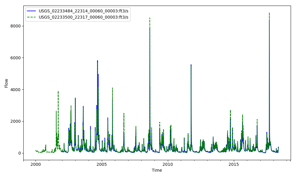
The default ‘tstoolbox plot …’ is a time-series plot where the datetime column is the x-axis, and all data columns are plotted on the y-axis.

tstoolbox read 02233484.csv,02233500.csv | tstoolbox plot --ofilename econ.png --columns USGS_02233484_22314_00060_00003:ft3/s,USGS_02233500_22317_00060_00003:ft3/s --ytitle Flow

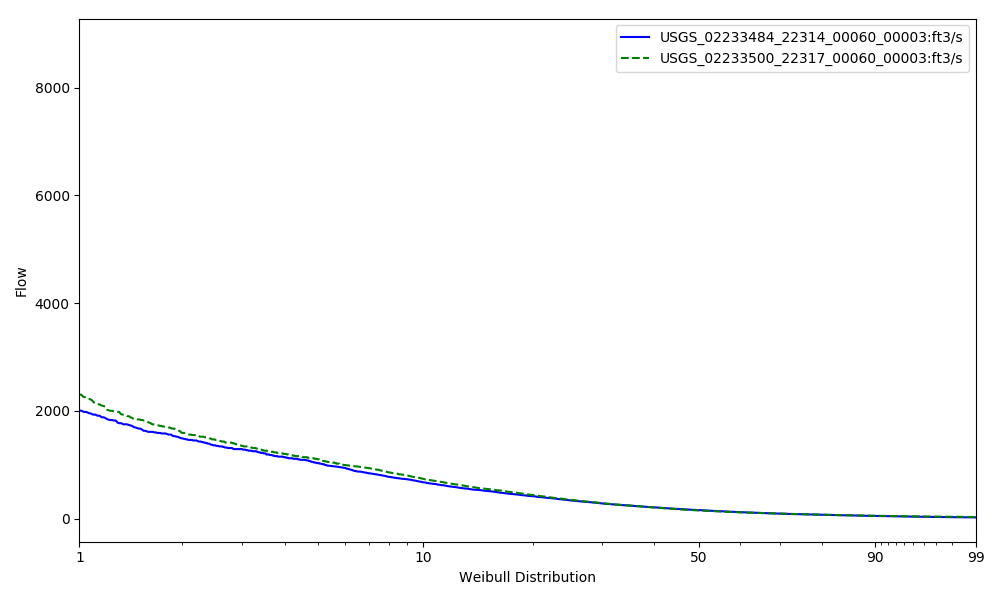
The ‘norm_xaxis’, ‘norm_yaxis’, ‘lognorm_xaxis’, ‘lognorm_yaxis’, ‘weibull_xaxis’, and ‘weibull_yaxis’ plot each data column against a transformed, sorted, ranking of the data.

For all of these plot types the datetime column is ignored.

tstoolbox read 02233484.csv,02233500.csv | tstoolbox plot --type weibull_xaxis --ofilename weibull.png --columns USGS_02233484_22314_00060_00003:ft3/s,USGS_02233500_22317_00060_00003:ft3/s --ytitle Flow

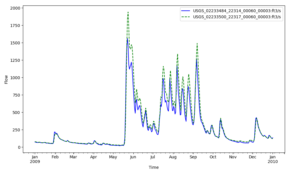
The following illustrates how to use the ‘–start_date ISO8601’ and ‘–end_date ISO8601’ to limit the x-axis of the plot.

tstoolbox read 02233484.csv,02233500.csv | tstoolbox plot --start_date 2009-01-01 --end_date 2010-01-01 --ofilename econ_clip.png --columns USGS_02233484_22314_00060_00003:ft3/s,USGS_02233500_22317_00060_00003:ft3/s --ytitle Flow

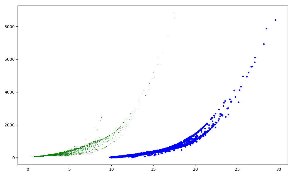
The ‘–type xy’ plot requires the data columns to be arranged ‘x1,y1,x2,y2,x3,y3,…’. You can use the ‘–columnns LIST’ option to rearrange or duplicate columns as needed. For example, if you have your data setup as ‘x,y1,y2,y3,…’, you can rearrage to what the ‘–type xy’ requires by ‘–columns 1,2,1,3,1,4,…’.

tstoolbox read 02233484.csv,02233500.csv | tstoolbox plot --type xy --ofilename econ_xy.png --columns 2,1,5,4 --linestyle ' ' --markerstyle auto

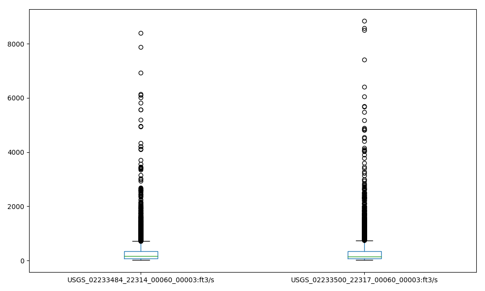
tstoolbox read 02233484.csv,02233500.csv | tstoolbox plot --type boxplot --ofilename boxplot.png --columns 1,4

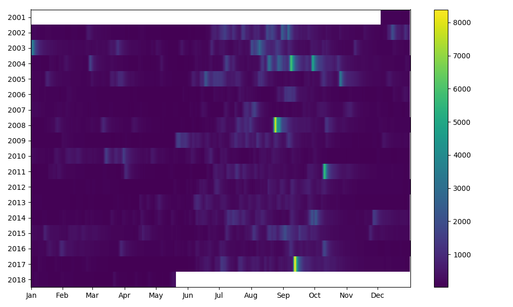
The ‘–type heatmap’ plot only work with a single, daily time-series. You can pick the series you want to plot using the ‘–columns INTEGER’ option.

tstoolbox plot --type heatmap --columns 1 --ofilename heatmap.png < 02233484.csv

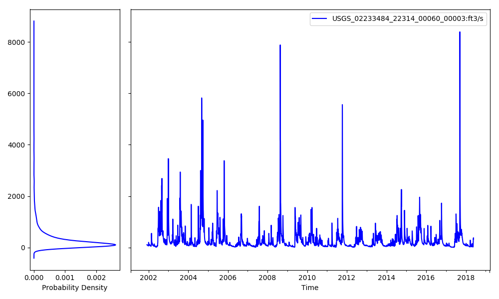
The ‘–type kde_time’ plot will make a time-series plot combined with a probability density plot. The probablity density plot is estimated using Kernel Density Estimation.

tstoolbox plot --type kde_time --columns 1 --ofilename kde_time.png < 02233484.csv